Some specific integrals
“Aber dann können sie’s!”
Two decades ago I was a math undergrad in Dresden, Germany.
At some point in the Analysis I course they taught us about solving integrals with the usual tricks: Integration by parts, substitution, partial fractions. Unlike physics or some engineering undergrads, math students would only see one or two examples and move on. I still remember my undergrad instructor Gerd Kayser telling us how this wasn’t proper training and how when he was a student, math undergrads in socialist East Germany had to do a preparatory course where they “had to solve 50 integrals”.
“50 integrals is a lot”, he said, “but we were told we shouldn’t complain since students in the Soviet Union have to solve 500. But afterwards they know how to solve integrals!”
The grace of my relatively late birth spared me having to do anywhere close that many and I never got good at it. The art of detecting if \(\tan\frac\theta 2\) is the right substitution continues to be lost on me.
In fact I was so bad at that sort of problem that my smart friends gave me a personalized set of integration exercises a few years later:
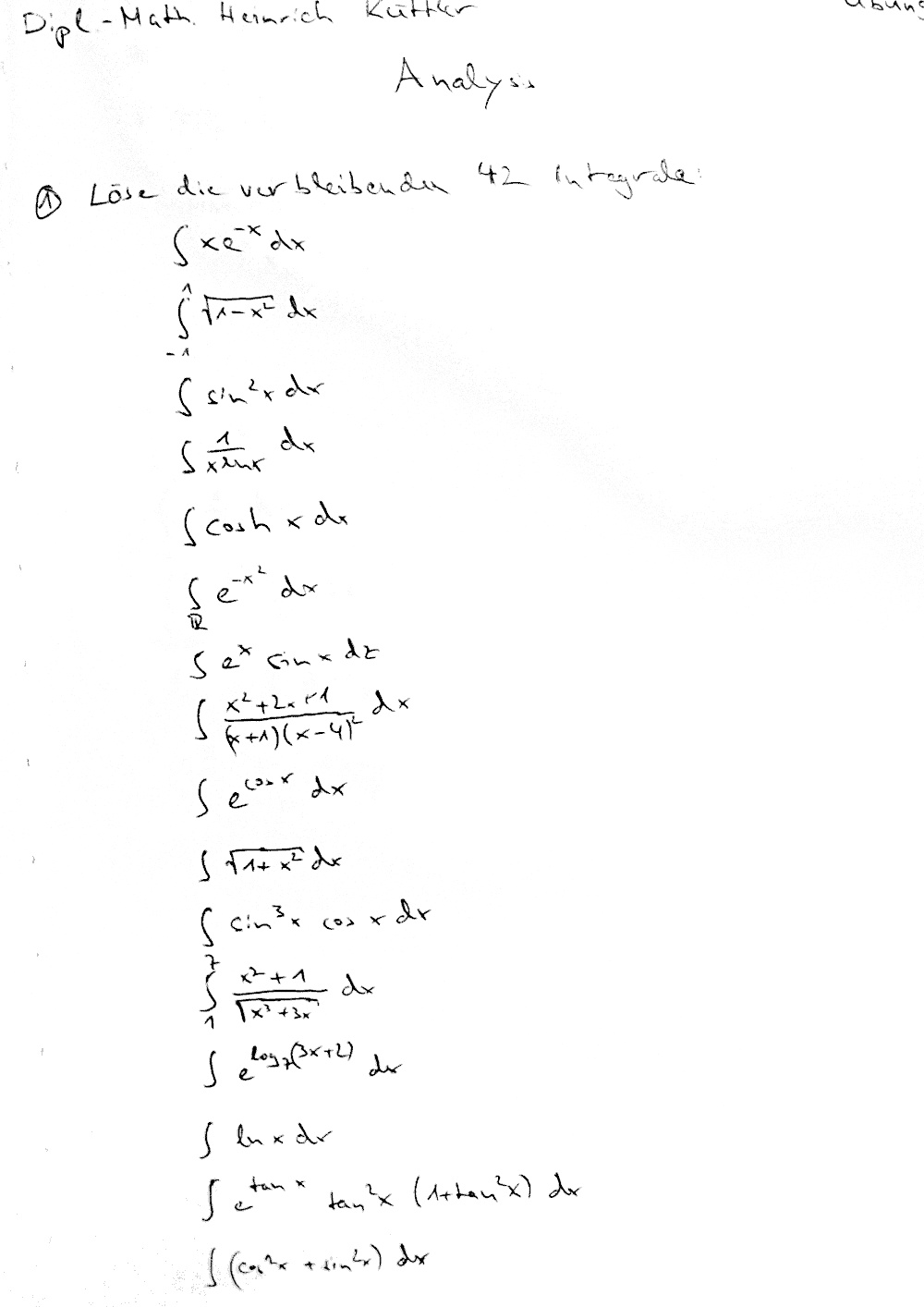
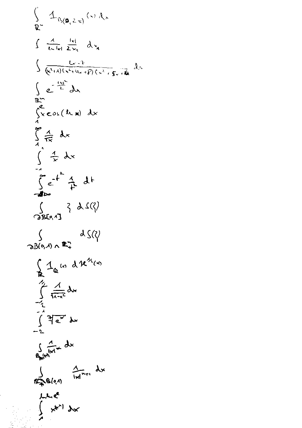
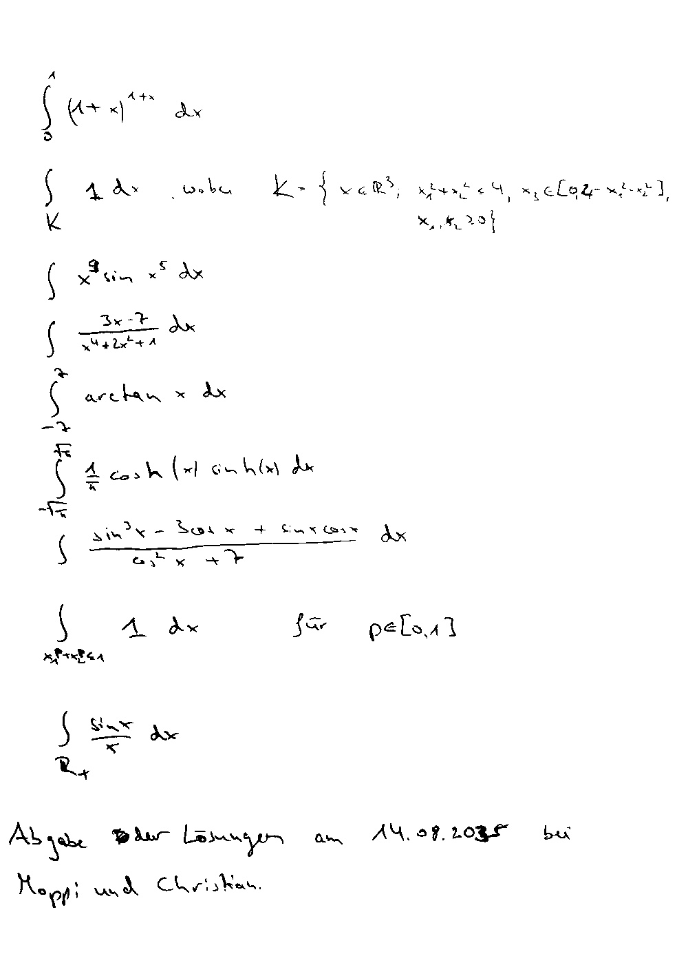
42 integrals to solve. I still got until 2035!
Lucky for me most of math isn’t about solving integrals. I eventually got my diploma and moved on.
Explicit but tricky
Moved on to doing a PhD in Mathematical Physics, that is. The quantum mechanical problem discussed in my thesis ultimately doesn’t matter1 but it turned out that after applying a trick by Feynman to each term of a certain series I was left with, ironically, an explicit integral that required solving!
Specifically, the \(n\)th term for \(n \ge 2\) produced the \(n\)-dimensional integral
\[I_n := \int_{(0,\infty)^n} \frac{e^{-\sum_{j=1}^n u_j}} {\prod_{j=1}^{n-1} (u_j + u_{j+1})}\d u\]where \((0,\infty)^n\) is the set of \(n\)-dimensional vectors \(u\in\R^n\) with positive entries \(u_j > 0\).
For small \(n\), I could solve this: \(I_2 = 1\), \(I_3 = \frac{\pi^2}{6}\), and \(I_4 = \frac{\pi^2}{3}\). I could also do numerics and find that \(I_5 \approx 7.3057 \approx \frac{3\pi^4}{40}\) and \(I_6 \approx 17.3172\approx\frac{8\pi^4}{45}\). But the iterated integrals turned complicated very quickly. Already for \(n=6\), the identity \(I_6 = \frac{8\pi^4}{45}\) turns out to be equivalent to the non-obvious dilogarithm integral
\[\int_0^1 \Bigl(\mathrm{Li}_2(\frac{x-1}{x})\Bigr)^2 \dx = \frac{17}{180}\pi^4\]for the dilogarithm \(\mathrm{Li}_2\). This is not exactly an obvious formula, although it turned out to be implied by results in the literature, which confirmed the value for \(n=6\).
Faith in math
The numerical results gave me a conjecture. It looked like \(I_{2n+2} = 2(2\pi)^{2n} \frac{(n!)^2}{(2n+2)!}\) might be correct.
When I plugged this result into my series expansion, the right power series coefficients (the one for \(\arcsin^2\)) would pop out and make the result of my thesis beautiful. The conjecture had to be true – the result was too good to be false!
How to prove it though?
I asked the internet but without receiving a super satisfactory result. However, after I massaged the integral a bit my collaborator Peter Otte found a solution using insights from operator theory, in particular Hankel operators.
The integral for all \(n\) turned out to be implied by results from the 1950s and earlier. To describe these, I have to go on a slight tangent.
An integral operator
On \(L_2(0, \infty)\), i.e., the space of functions from the half-line \((0, \infty)\) to the reals that are square-integrable, define an operator \(L_2(0, \infty) \ni f \mapsto Tf \in L_2(0,\infty)\), i.e., a mapping from functions to functions, by
\[(Tf)(x) = \int_0^\infty \frac{e^{-(x+y)/2}}{x+y}f(y)\,\d y.\]This is an integral operator of the form \((Tf)(x) = \int k(x, y) f(y)\,\d y\). The function \(k(x, y)\) is called a kernel. In this particular case, the kernel depends on \(x+y\) only, not on \(x\) and \(y\) separately. Such operators are known as Hankel operators.
The reason the operator \(T\) is interesting vis-à-vis the integral \(I_n\) is that applying it repeatedly yields iterated integrals that look like \(I_n\). In fact,
\[I_n = \langle \varphi, T^{n-1} \varphi \rangle\]where \(\langle \dotid, \dotid\rangle\) is the scalar product on \(L_2(0, \infty)\) and \(\varphi(x) := e^{-x/2}\).
It turns out that the operator \(T\) has been studied by mathematicians. Rosenblum (1958) gave an explicit diagonalization of this operator. Diagonalization is part of the spectral analysis of an operator, a powerful concept that involves finding the fundamental properties of the operator as a mathematical object (finding out all its secrets, as it were). Like its finite-dimensional analog matrix diagonalization, it allows us to compute “functions of the operator”, including its powers \(T^n\).
The diagonalization of \(T\) due to Rosenblum can be written as \begin{equation} \label{eq:Hilbert-matrix-unitary-relation} (UTf)(k) = \frac{\pi}{\cosh(k\pi)}(Uf)(k) \where{k\in(0,\infty), f\in L_2(0,\infty)} \end{equation} for a specific unitary operator \(U\from L_2(0,\infty)\to L_2(0,\infty)\). Unitary means that \(U\) is a Hilbert space isomorphism, i.e. it maps the Hilbert space \(L_2(0,\infty)\) to itself while leaving its structure in place; in particular the scalar product of two mapped functions is the same as the scalar product of the input functions. The operator \(U\) can be explicitly computed although the details are a bit messy and require a number of functions from the special functions zoo (the Gamma function and the Whittaker functions). If you must know the details you can check out chapter 8 of my thesis.
Using these results, my integral expression can be turned into something much more manageable, because with \(\hat{\varphi} := U\varphi\) one has
\[I_n = \langle \varphi, T^{n-1} \varphi \rangle = \langle U\varphi, UT^{n-1} \varphi \rangle = \int_0^\infty\d k\, \abs{\hat{\varphi}(k)}^2 \Big(\frac{\pi}{\cosh(k\pi)}\Big)^{n-1}\]by repeated application of Rosenblum’s diagonalization.
The function \(\hat{\varphi}\) and the remaining one-dimensional integral can be computed, and the result is
\[I_n = \frac{2}{n}(2\pi)^{n-2} \frac{\bigl(\Gamma(\frac{n}{2})\bigr)^2}{\Gamma(n)},\]in particular \(I_{2n+2} = 2(2\pi)^{2n} \frac{(n!)^2}{(2n+2)!}\), my conjecture! My faith wasn’t misplaced; by faith we understand the universe.
More?
These kinds of explicit integral expressions are somewhat unusual in research mathematics. In fact, some follow-up work by other mathematicians lightly criticized our approach as “curious”.
But I had fun with my integral. Just not enough fun to stay in research mathematics.
My co-author Martin Gebert pushed the underlying physics question much further. Curiously, that yielded more interesting integrals, one of which I’ll describe below.
The Hilbert Matrix
As an aside, the Rosenblum operator \(T\) turns out to show up in other disguises. For instance, the “infinite matrix”
\[H = \begin{pmatrix} 1 & \frac{1}{2} & \frac{1}{3} & \frac{1}{4} & \cdots \\ \frac{1}{2} & \frac{1}{3} & \frac{1}{4} & \iddots \\ \frac{1}{3} & \frac{1}{4} & \iddots \\ \frac{1}{4} & \iddots \\ \vdots \end{pmatrix}\]is known as the Hilbert matrix. Its entries at position \(j, k\) are \(\frac{1}{j + k - 1}\). In numerical analysis, it usually serves as a cautionary tale about ill-conditioned systems.
Since the entries depend only on \(j+k\), they are constant along the anti-diagonals. Matrices with this property are called Hankel matrices. The Hilbert matrix is the most famous example; below we will see others.
On the space \(\ell_2(\N)\) of square-summable sequences, it turns out this matrix is unitarily equivalent (aka essentially the same under a Hilbert space isomorphism) to Rosenblum’s integral operator \(T\).2
Lots of beautiful mathematics and hidden connections lurk behind these objects.
The Dirichlet integral
The improper integral
\[\int_0^\infty \frac{\sin x}{x} \d x = \frac{\pi}{2}\]is a well-known classical result known as the Dirichlet integral. It’s also the final integral exercise in the above list of 42 integrals to solve.
Dirichlet’s integral is “improper” in the sense that the integrand \(\sinc(x) = \frac{\sin x}{x}\) isn’t actually integrable (the integral \(\int_0^\infty \abs{\sinc(x)}\d x\) isn’t finite). While the specific limit \(\lim_{L\to\infty}\int_0^L \sinc(x)\d x\) exists, that is due to cancellation from the sign change of \(\sin\). This cancellation depends on how the limit is done; this makes \(\sinc\) not Lebesgue-integrable on unbounded intervals.
Proof via Laplace transform. One way to prove Dirichlet’s identity is to use an Abelian theorem which in this form is also known as the “final value theorem” of the Laplace transform. It states that if the limit \(\lim_{L\to\infty} \int_0^L \frac{\sin x}{x}\d x\) exists, its value is the same as the limit of the regularization of its integrand via the Laplace transform3
\[\lim_{s \downarrow 0} \int_0^\infty e^{-st} \frac{\sin(t)}{t} \d t.\]This expression can be evaluated for \(s > 0\) with Laplace transform tricks (essentially differentiating by \(s\) to turn this into the Laplace transform of \(\sin\) itself). Its value turns out to be \(\frac{\pi}{2} - \arctan s\) and the \(\arctan\) term goes to zero as \(s\to 0\).
This used an “Abelian theorem” which requires the existence of the original limit as one of its ingredients. In this case, the existence is provided by, appropriately enough, Dirichlet’s test.
It’s also an example of a common pattern in mathematics (which is also the main approach in my PhD thesis): The quantity of interest is not quite well behaved, but it’s the limit of well-behaved expressions. So one does a “regularization” (in this case the Laplace transform) which turns it into a well-behaved expression, does the required calculations there, then goes back to something like the original. There is extra work involved in doing and undoing the regularization, but the benefit is that the main work can be done in a better space.
With some help by ChatGPT, I recently learned about a less common proof for Dirichlet’s identity which turned out to be directly generalizable to another related tricky \(n\)-dimensional integral. Instead of an Abelian theorem, it uses Cauchy’s integral theorem and an explicit calculation with hyperbolic functions. Since it’s somewhat fun, I’ll write it down here. This proof might look a bit lengthy, but like Wagner’s music it’s not as bad as it sounds:
Proof via Cauchy’s integral theorem. Set \(I(L) := \int_0^L \frac{\sin x}{x}\d x\). Since \(\frac{\sin y}{y}=\frac12\int_{-1}^{1}e^{ity}\,dt,\) Fubini and the substitution \(t = \tanh(s/2)\) where \(\d t = w(s) \d s\) for \(w(s) = \frac{1}{2}\sech^2(s/2)\) give
\[I(L) = \frac{1}{2}\int_{-1}^1 \int_0^L e^{ixt}\,\d x \,\d t = \frac{1}{2}\int_{-1}^1 D_L(t)\,\d t = \frac{1}{2}\int_\R w(s) D_L(\tanh\tfrac{s}{2}) \,\d s\]with \(D_L(t) := \int_0^L e^{ixt}\,\dx = \frac{e^{iLt} - 1}{it}\) where \(D_L(0) := L\) makes this function entire.
Now, shift the domain of integration from \(\R\) to \(\R + i\pi/2\) via Cauchy’s integral theorem. For \(R > 0\) we will use expanding boxes \([-R, R] + i[0, \frac{\pi}{2}]\) on the complex plane. On the full strip \(0 \le \Im z \le \frac{\pi}{2}\) all functions involved are holomorphic and therefore
\[\int_{-R}^R w(s) D_L(\tanh\tfrac{s}{2}) \,\d s + \int_0^{\pi/2} w(R+i\beta) D_L(\tanh(\tfrac{R+i\beta}{2})) \,\d\beta = \int_{-R}^R w(s + i\tfrac{\pi}{2}) D_L(\tanh(\tfrac{s}{2} + i\tfrac{\pi}{4})) \,\d s + \int_0^{\pi/2} w(-R+i\beta) D_L(\tanh(\tfrac{-R+i\beta}{2})) \,\d\beta.\]Now, since
\[\Im\tanh(\tfrac{s+i\beta}{2}) = \frac{\sin\beta}{\cosh s + \cos\beta} \ge 0,\]we have \(\abs{D_L(\tanh z)} \le L\) anywhere on the strip. On the vertical sides of the box, one has
\[\abs{w(\pm R + i\beta)} = \frac{1}{\cosh R + \cos\beta} \le \frac{1}{\cosh R} = \sech R \to 0 \where{R\to\infty}.\]So the vertical parts of the contour vanish in the \(R\to\infty\) limit, and
\[I(L) = \frac{1}{2}\int_\R w(s + i\tfrac{\pi}{2}) D_L(\tanh(\tfrac{s}{2} + i\tfrac{\pi}{4})) \,\d s.\]We have shifted the integration domain up by \(\pi/2\) in the complex plane without changing the value of the integral. This had the effect of making the functions \(D_L\) well-behaved: For \(\Im z > 0\) we have both \(\abs{D_L(z)} \le \frac{2}{\abs{z}}\) and \(D_L(z) \to \frac{i}{z}\) as \(L\to\infty\). Additionally
\[\frac{w(z)}{\tanh(z/2)} = \frac{1}{\sinh z}.\]Since \(\tanh(\tfrac{s}{2} + i\tfrac{\pi}{4}) = \frac{\sinh s + i}{\cosh s} = \tanh s + i \sech s\) and \(\sech s > 0\), this bounds the integrand by
\[\frac{2}{\abs{\sinh(s + i\pi/2)}} = \frac{2}{\cosh s}\]which is integrable, so the dominated convergence theorem gives
\[\lim_{L\to\infty} I(L) = \frac{i}{2}\int_\R \frac{\d s}{\sinh(s + i\pi/2)} = \frac{i}{2}\int_\R\frac{\d s}{i\cosh s} = \frac{1}{2}\int_\R\sech s \,\d s = \frac{1}{2}\arctan(\sinh s) \Bigr\rvert_{s=-\infty}^\infty = \frac{\pi}{2}.\]A generalization of the Dirichlet integral
It turns out that in connection to the same quantum mechanical phenomenon that led to the \(I_n\) integral, the cyclic integral
\[S_n = \lim_{L\to\infty} \int_{(0, L)^n} \prod_{j=1}^n \frac{\sin(x_j + x_{j+1})}{x_j + x_{j+1}} \,\d x \where{n \in 2\N + 1}\]pops up, where \(x_{n+1} := x_1\). Some time after Martin Gebert showed me this, I could show \(S_3 = \frac{\pi^3}{16}\) using a Laplace transform in a somewhat lengthy Stack Exchange answer. But that method doesn’t extend to general odd \(n\). From numerics, the conjecture \(S_n = \frac{\pi^n}{2^{n+1}}\) seemed likely.
I attempted to apply Hankel operator diagonalizations from the literature. That seemed tempting because it worked for \(I_n\) and the operator with \(\sinc\) kernel is understood in the literature – it’s been studied by Krein and others and while it’s not well-behaved (in particular, it’s not trace class, or even compact), it is the limit of well-behaved operators. The integral \(S_n\) is the limit of a sequence of traces of operators. The limit operator is closely related to the Rosenblum operator / Hilbert matrix from \(I_n\).
Viewing it as a trace is also the approach most LLMs go for when asked this question.4
I tried operator theoretic approaches for a while and learned a good deal about Hankel operators and Hardy spaces. But I did not manage to make real headway with this. Since the limit isn’t trace class, most usual tools don’t apply and regularizations of the operator were too complicated for me to do enough analysis on.
I will still describe some of the math I learned since I found it interesting and to show why Hankel operators looked tempting for this problem. The actual solution for \(S_n\) (in the final section below) turned out to be more elementary.
More Hankel matrices and operators
Above, we learned that Rosenblum’s operator relates to the Hilbert matrix:
Hilbert matrix and Rosenblum’s operator
\[\frac{1}{\pi}\begin{pmatrix} 1 & \frac{1}{2} & \frac{1}{3} & \frac{1}{4} & \cdots \\ \frac{1}{2} & \frac{1}{3} & \frac{1}{4} & \iddots \\ \frac{1}{3} & \frac{1}{4} & \iddots \\ \vdots \end{pmatrix} \quad\longleftrightarrow\quad \frac{1}{\pi}\int_0^\infty \frac{e^{-(x+y)/2}}{x+y} f(y) \, \d y\]With a \(\frac{1}{\pi}\) normalization, this operator has spectrum \([0, 1]\).
Carleman operator
If we take the Hilbert matrix but put zeros into every other anti-diagonal, it becomes unitarily equivalent to the Carleman operator \(\int_0^\infty \frac{f(y)}{x+y}dy\). Power (1980) shows this via a chain of equivalences through the Hardy spaces \(H_2(\R)\) and \(H_2(\C_{\Im>0})\):
\[\frac{2}{\pi} \begin{pmatrix} 1 & 0 & \frac{1}{3} & 0 & \frac{1}{5} \\ 0 & \frac{1}{3} & 0 & \frac{1}{5} & \iddots \\ \frac{1}{3} & 0 & \frac{1}{5} & \iddots \\ \vdots \end{pmatrix} \quad\longleftrightarrow\quad \frac{1}{\pi}\int_0^\infty \frac{1}{x+y} f(y) \, \d y\]Carleman’s (1923) original work shows its spectrum is \([0, 1]\).
Krein’s example
The operator involved in \(S_n\) was studied by Krein and others. One interesting read is “On Krein’s example” by Kostrykin and Makarov (2006), where they show that it’s the Carleman operator with alternating signs for each anti-diagonal:
\[\frac{2}{\pi}\begin{pmatrix} \phantom{-}1 & \phantom{-}0 & -\frac{1}{3} & 0 & \frac{1}{5} \\ \phantom{-}0 & -\frac{1}{3} & \phantom{-}0 & \frac{1}{5} & \iddots \\ -\frac{1}{3} & \phantom{-}0 & \phantom{-}\frac{1}{5} & \iddots \\ \vdots \end{pmatrix} \quad\longleftrightarrow\quad \frac{2}{\pi}\int_0^\infty \frac{\sin(x+y)}{x+y} f(y) \, \d y\]The paper shows its spectrum is \([-1, 1]\). They study it in connection with a perturbation problem, but the sinc kernel \(\frac{\sin(x+y)}{x+y}\) also shows up in random matrix theory and many other places.
Hilbert space equivalences
I found it interesting how the various Hilbert spaces involved relate to each other. The core idea is that via Fourier series, series in \(\ell_2(\Z)\) or \(\ell_2(\N_0)\) relate to periodic functions, which can be viewed as functions on the unit circle \(\T = \set{z\in\C\st \abs{z}=1}\). These in turn can sometimes be extended to the full unit ball. The Moebius transform turns them into functions of the real line or upper half-plane and the Fourier transform maps them to where the integral operators live:
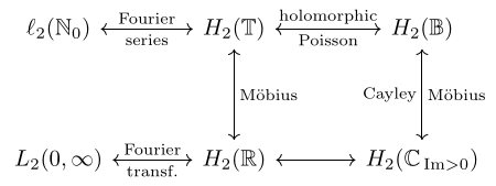
The relevant subspaces of functions of the unit circle and unit ball are the Hardy spaces.5
The actual solution for \(\int_{(0, \infty)^n} \prod_{j=1}^n \frac{\sin(x_j + x_{j+1})}{x_j + x_{j+1}} \d x\)
It’s 2026 and LLMs are now truly useful for mathematics. The main bottleneck is that their proofs are still often wrong, too complicated, or incomplete. Carefully verifying their output is at this point still required and often tedious.
However, I found that ChatGPT 5.5 Extended Pro was eventually able to give me something useful for the \(S_n\) integral. Its first several approaches were both handwavy and complicated, but after I confronted it with its own shortcomings often enough it produced the outline of a correct and elementary proof.
The same approach of moving the integration domain into the complex plane using Cauchy’s integral theorem that shows the Dirichlet integral identity above turns out to work for \(S_n\). (In fact, I wrote the Dirichlet integral solution after that approach solved \(S_n\).) Using \(\frac{\sin y}{y}=\frac12\int_{-1}^{1}e^{ity}\,dt\) and the substitution \(t = \tanh(s/2)\) one can shift the contour up by \(\pi/2\). For odd \(n\), the \(L\to\infty\) limit then turns into a product of \(\sech\) integrals. The conjecture \(S_n = \frac{\pi^n}{2^{n+1}}\) is correct. For the details, see this Stack Exchange answer.6
Given that \(I_n\) and \(S_n\) are really a countably infinite number of integrals, I believe I finally did enough integrals now.
Bibliography
- T. Carleman, Sur les équations intégrales singulières à noyau réel et symétrique, Almqvist and Wiksell, Uppsala, 1923. (Introduces and analyzes the \(\frac{1}{\pi(x+y)}\) operator; determines its spectrum as \([0,1]\).)
- D. Hilbert, “Ein Beitrag zur Theorie des Legendre’schen Polynoms,” Acta Mathematica 18 (1894), 155–159. (Original appearance of the Hilbert matrix.)
- H. Küttler, “Anderson’s Orthogonality Catastrophe,” dissertation, Ludwig-Maximilians-Universität München, 2014.
- V. Kostrykin and K. A. Makarov, “On Krein’s example,” arXiv:math/0606249 (2006). (Proves the sinc-kernel operator \(K_\mu\) has purely absolutely continuous spectrum \([-1,1]\); makes the connection to Hankel operator theory via Power’s results explicit.)
- S. C. Power, “Hankel operators on Hilbert space,” Bulletin of the London Mathematical Society 12 (1980), 422–442. (Excellent survey; contains the explicit unitary equivalence chain from the alternating matrix to Carleman’s operator.)
- M. Rosenblum, “On the Hilbert matrix, I,” Proceedings of the American Mathematical Society 9 (1958), 137–140. (Identifies the \(L_2(0,\infty)\) operator via Laguerre functions and Whittaker functions.)
-
If you need to know, Anderson’s orthogonality catastrophe — a phenomenon where the ground states of a Fermi gas before and after a tiny perturbation become orthogonal to each other as the system grows large. The overlap between them decays as a power law, and expanding the exponent into a series expression produced the integral \(I_n\) for the \(n\)th term. But you don’t actually need to know any of that. ↩
-
The orthonormal basis of \(L_2(0,\infty)\) that makes this correspondence to the Hilbert matrix work is given by the weighted Laguerre polynomials \(\phi_n(x) = e^{-x/2}L_n(x)\). ↩
-
The Laplace transform and Abelian and Tauberian theorems for it also underlie the proof of the prime number theorem which involves controlling certain expressions involving Riemann’s \(\zeta\) function. ↩
-
E.g., Opus 4.8 approaches this as traces of operators. Fable 5 eventually tried another approach, but it was also complicated and incomplete. ↩
-
Incidentally, it’s a more complicated version of Hardy spaces that Louis de Branges tried to use in his claimed proof for the famous Riemann hypothesis. I found this writeup somewhat interesting, and the relevant section of Wikipedia almost hilarious. ↩
-
In fact, ChatGPT also can do the original integral \(I_n\) in a more elementary way when asked. ↩